Logistic Regression

Basically, logistic regression model is one of the members of supervised classification algorithm family. Logistic regression measures the relationship between dependent variables and independent variables by estimating the probabilities using a logistic function.

Here, if we talk about dependent and independent variables then dependent variable is the target class variable we are going to predict and on the other side the independent variables are the features we are going to use to predict the target class.

In logistic regression, estimating the probabilities means to predict the likelihood occurrence of the event. For example, the shop owner would like to predict the customer who entered into the shop will buy the play station (for example) or not. There would be many features of customer − gender, age, etc. which would be observed by the shop keeper to predict the likelihood occurrence, i.e., buying a play station or not. The logistic function is the sigmoid curve that is used to build the function with various parameters.

Prerequisites
Before building the classifier using logistic regression, we need to install the Tkinter package on our system. It can be installed from https://docs.python.org/2/library/tkinter.html.

Now, with the help of the code given below, we can create a classifier using logistic regression −

First, we will import some packages −

import numpy as np
from sklearn import linear_model
import matplotlib.pyplot as plt
Now, we need to define the sample data which can be done as follows −

X = np.array([[2, 4.8], [2.9, 4.7], [2.5, 5], [3.2, 5.5], [6, 5], [7.6, 4],
              [3.2, 0.9], [2.9, 1.9],[2.4, 3.5], [0.5, 3.4], [1, 4], [0.9, 5.9]])
y = np.array([0, 0, 0, 1, 1, 1, 2, 2, 2, 3, 3, 3])
Next, we need to create the logistic regression classifier, which can be done as follows −

Classifier_LR = linear_model.LogisticRegression(solver = 'liblinear', C = 75)
Last but not the least, we need to train this classifier −

Classifier_LR.fit(X, y)
Now, how we can visualize the output? It can be done by creating a function named Logistic_visualize() −

Def Logistic_visualize(Classifier_LR, X, y):
   min_x, max_x = X[:, 0].min() - 1.0, X[:, 0].max() + 1.0
   min_y, max_y = X[:, 1].min() - 1.0, X[:, 1].max() + 1.0
In the above line, we defined the minimum and maximum values X and Y to be used in mesh grid. In addition, we will define the step size for plotting the mesh grid.

mesh_step_size = 0.02
Let us define the mesh grid of X and Y values as follows −

x_vals, y_vals = np.meshgrid(np.arange(min_x, max_x, mesh_step_size),
                 np.arange(min_y, max_y, mesh_step_size))
With the help of following code, we can run the classifier on the mesh grid −

output = classifier.predict(np.c_[x_vals.ravel(), y_vals.ravel()])
output = output.reshape(x_vals.shape)
plt.figure()
plt.pcolormesh(x_vals, y_vals, output, cmap = plt.cm.gray)

plt.scatter(X[:, 0], X[:, 1], c = y, s = 75, edgecolors = 'black',
linewidth=1, cmap = plt.cm.Paired)
The following line of code will specify the boundaries of the plot

plt.xlim(x_vals.min(), x_vals.max())
plt.ylim(y_vals.min(), y_vals.max())
plt.xticks((np.arange(int(X[:, 0].min() - 1), int(X[:, 0].max() + 1), 1.0)))
plt.yticks((np.arange(int(X[:, 1].min() - 1), int(X[:, 1].max() + 1), 1.0)))
plt.show()

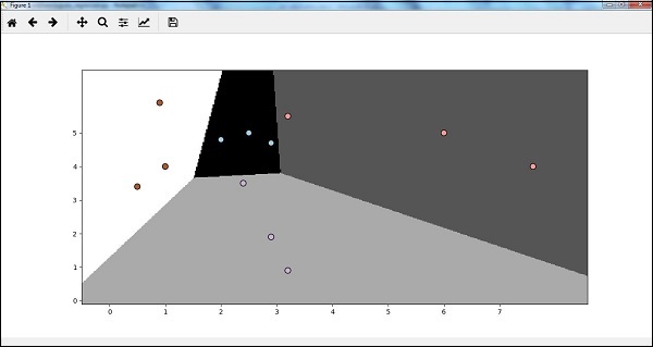
Now, after running the code we will get the following output, logistic regression classifier −